38 excel line graph axis labels
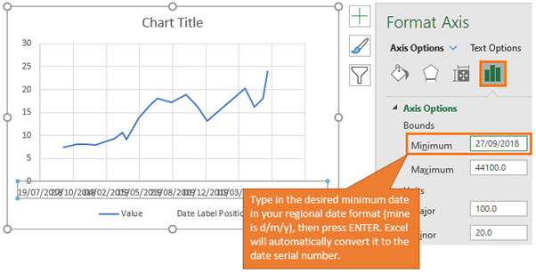
How to Make Line Graphs in Excel | Smartsheet Excel creates the line graph and displays it in your worksheet. Other Versions of Excel: Click the Insert tab > Line Chart > Line. In 2016 versions, hover your cursor over the options to display a sample image of the graph. Customizing a Line Graph To change parts of the graph, right-click on the part and then click Format. Excel charts: add title, customize chart axis, legend and data labels Click the arrow next to Axis, and then click More options… This will bring up the Format Axis pane. 3. On the Format Axis pane, under Axis Options, click the value axis that you want to change and do one of the following: To set the starting point or ending point for the vertical axis, enter the corresponding numbers in the Minimum or Maximum
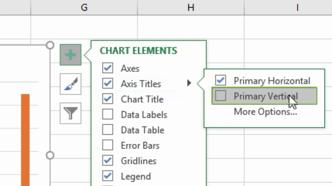
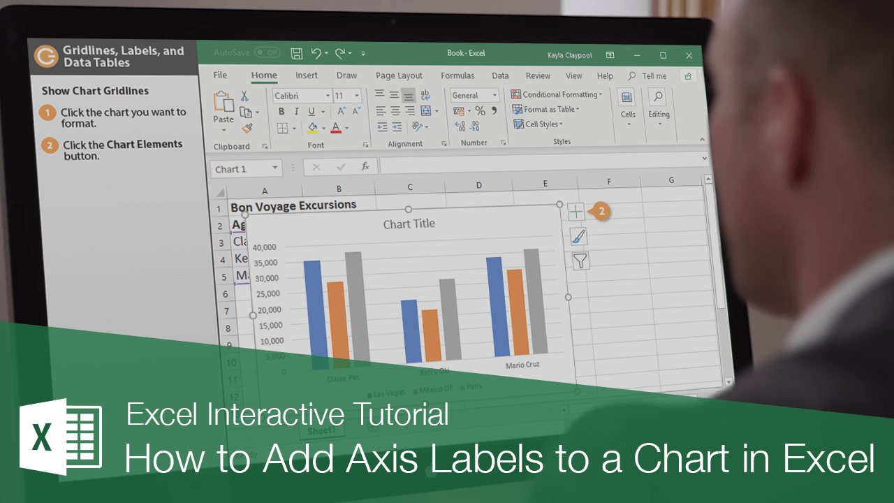
How to Label Axes in Excel: 6 Steps (with Pictures) - wikiHow Select the graph. Click your graph to select it. 3 Click +. It's to the right of the top-right corner of the graph. This will open a drop-down menu. 4 Click the Axis Titles checkbox. It's near the top of the drop-down menu. Doing so checks the Axis Titles box and places text boxes next to the vertical axis and below the horizontal axis.

Excel line graph axis labels
How to rotate axis labels in chart in Excel? - ExtendOffice If you are using Microsoft Excel 2013, you can rotate the axis labels with following steps: 1. Go to the chart and right click its axis labels you will rotate, and select the Format Axis from the context menu. 2. Shorten Y Axis Labels On A Chart - How To Excel At Excel Right-click the Y axis (try right-clicking one of the labels) and choose Format Axis from the resulting context menu. Choose Number in the left pane. In Excel 2003, click the Number tab. Choose Custom from the Category list. Enter the custom format code £0,,\ m, as shown in Figure 2. In Excel 2007, click Add. 3 Types of Line Graph/Chart: + [Examples & Excel Tutorial] - Formpl 20.04.2020 · Labels. Each axis on a line graph has a label that indicates what kind of data is represented in the graph. The X-axis describes the data points on the line and the y-axis shows the numeric value for each point on the line. We have 2 types of labels namely; the horizontal label and the vertical label. The horizontal label defines the data that is being described on the x …
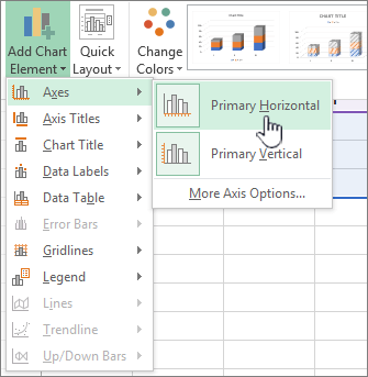
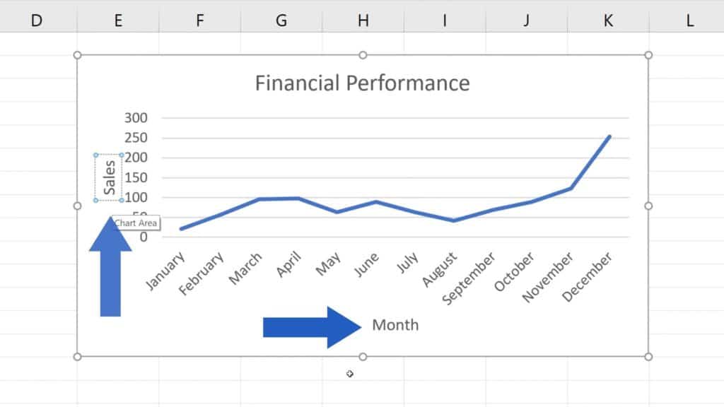
Excel line graph axis labels. How to Add X and Y Axis Labels in Excel (2 Easy Methods) Then go to Add Chart Element and press on the Axis Titles. Moreover, select Primary Horizontal to label the horizontal axis. In short: Select graph > Chart Design > Add Chart Element > Axis Titles > Primary Horizontal. Afterward, if you have followed all steps properly, then the Axis Title option will come under the horizontal line. How to add Axis Labels (X & Y) in Excel & Google Sheets Adding Axis Labels Double Click on your Axis Select Charts & Axis Titles 3. Click on the Axis Title you want to Change (Horizontal or Vertical Axis) 4. Type in your Title Name Axis Labels Provide Clarity Once you change the title for both axes, the user will now better understand the graph. Create a Line Chart in Excel (In Easy Steps) - Excel Easy Line charts are used to display trends over time. Use a line chart if you have text labels, dates or a few numeric labels on the horizontal axis. Use a scatter plot (XY chart) to show scientific XY data. To create a line chart, execute the following steps. 1. Select the range A1:D7. 2. On the Insert tab, in the Charts group, click the Line symbol. How to Insert Axis Labels In An Excel Chart | Excelchat We will go to Chart Design and select Add Chart Element Figure 6 - Insert axis labels in Excel In the drop-down menu, we will click on Axis Titles, and subsequently, select Primary vertical Figure 7 - Edit vertical axis labels in Excel Now, we can enter the name we want for the primary vertical axis label.
How to make a 3 Axis Graph using Excel? - GeeksforGeeks 20.06.2022 · Step 1: Select table B3:E12.Then go to Insert Tab, and select the Scatter with Chart Lines and Marker Chart.. Step 2: A Line chart with a primary axis will be created. Step 3: The primary axis of the chart will be Temperature, the secondary axis will be Pressure and the third axis will be Volume.So, to create the third axis duplicate this chart by pressing Ctrl + D while … How to display text labels in the X-axis of scatter chart in Excel? Display text labels in X-axis of scatter chart Actually, there is no way that can display text labels in the X-axis of scatter chart in Excel, but we can create a line chart and make it look like a scatter chart. 1. Select the data you use, and click Insert > Insert Line & Area Chart > Line with Markers to select a line chart. See screenshot: 2. 10 Design Tips to Create Beautiful Excel Charts and Graphs in 2021 24.09.2015 · Excel Design Tricks for Sprucing Up Ugly Charts and Graphs in Microsoft Excel 1) Pick the right graph. Before you start tweaking design elements, you need to know that your data is displayed in the optimal format. Bar, pie, and line charts all tell different stories about your data -- you need to choose the best one to tell the story you want. How to Place Labels Directly Through Your Line Graph in Microsoft Excel ... Select Format Data Labels. In the Format Data Labels editing window, adjust the Label Position. By default the labels appear to the right of each data point. Click on Center so that the labels appear right on top of each point. Umm yeah. So the labels are totally unreadable because they've got a line running through them.
How to wrap X axis labels in a chart in Excel? - ExtendOffice And you can do as follows: 1. Double click a label cell, and put the cursor at the place where you will break the label. 2. Add a hard return or carriages with pressing the Alt + Enter keys simultaneously. 3. Add hard returns to other label cells which you want the labels wrapped in the chart axis. Add a Horizontal Line to an Excel Chart - Peltier Tech 11.09.2018 · We can change the Axis Position to On Tick Marks, below, and the first and last category labels line up with the ends of the category axis. The line chart looks okay, but we have cut off the outer halves of the first and last columns. Let’s focus on a column chart (the line chart works identically), and use category labels of 1 through 5 instead of A through E. Excel doesn’t … How to add a line in Excel graph: average line, benchmark, etc. Tips: The same technique can be used to plot a median For this, use the MEDIAN function instead of AVERAGE.; Adding a target line or benchmark line in your graph is even simpler. Instead of a formula, enter your target values in the last column and insert the Clustered Column - Line combo chart as shown in this example.; If none of the predefined combo charts suits your needs, select the ... How to move Excel chart axis labels to the bottom or top - Data Cornering Move Excel chart axis labels to the bottom in 2 easy steps Select horizontal axis labels and press Ctrl + 1 to open the formatting pane. Open the Labels section and choose label position " Low ". Here is the result with Excel chart axis labels at the bottom. Now it is possible to clearly evaluate the dynamics of the series and see axis labels.
How To Add Axis Labels In Excel - BSUPERIOR
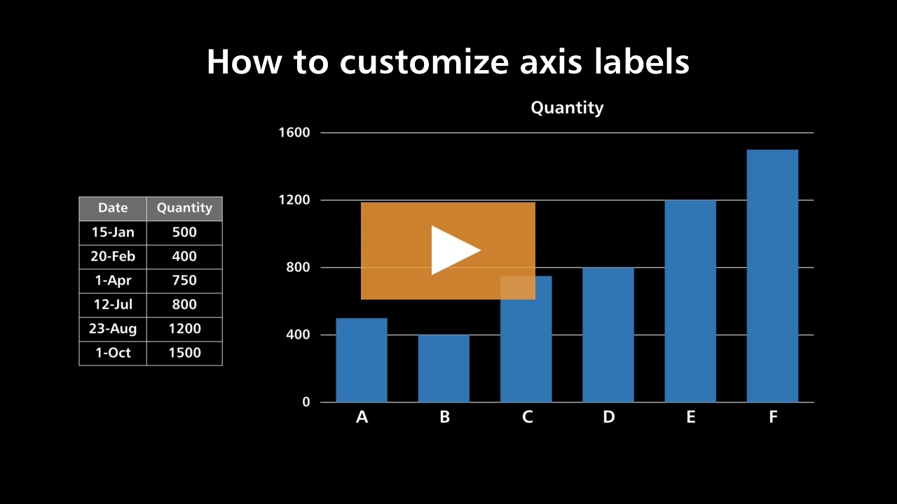
Excel tutorial: How to customize axis labels Instead you'll need to open up the Select Data window. Here you'll see the horizontal axis labels listed on the right. Click the edit button to access the label range. It's not obvious, but you can type arbitrary labels separated with commas in this field. So I can just enter A through F. When I click OK, the chart is updated.
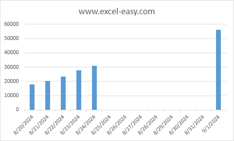
Chart Axes in Excel - Easy Tutorial
How to Make Charts and Graphs in Excel | Smartsheet Jan 22, 2018 · The seven line chart options are line, stacked line, 100% stacked line, line with markers, stacked line with markers, 100% stacked line with markers, and 3-D line. Scatter Charts: Similar to line graphs, because they are useful for showing change in variables over time, scatter charts are used specifically to show how one variable affects another.
Change the display of chart axes
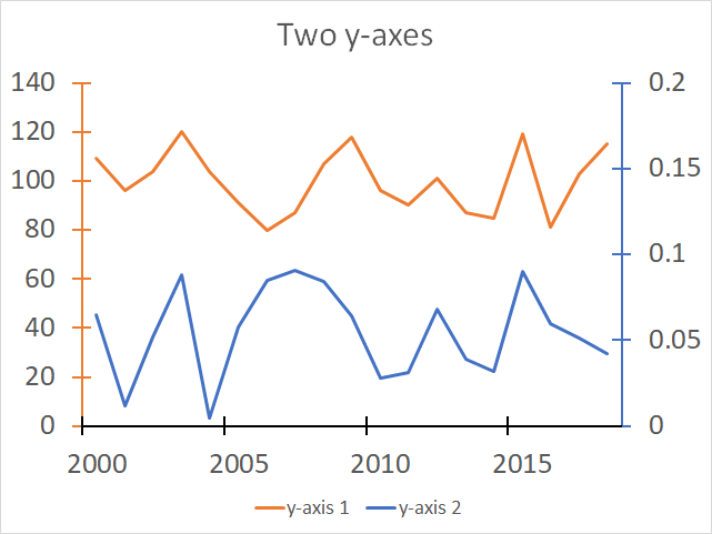
Add or remove a secondary axis in a chart in Excel After you add a secondary vertical axis to a 2-D chart, you can also add a secondary horizontal (category) axis, which may be useful in an xy (scatter) chart or bubble chart. To help distinguish the data series that are plotted on the secondary axis, you can change their chart type. For example, in a column chart, you could change the data ...

Dynamically Label Excel Chart Series Lines • My Online ...
How to create a chart with date and time on X axis in Excel? To display the date and time correctly, you only need to change an option in the Format Axis dialog. 1. Right click at the X axis in the chart, and select Format Axis from the context menu. See screenshot: 2. Then in the Format Axis pane or Format Axis dialog, under Axis Options tab, check Text axis option in the Axis Type section. See screenshot:
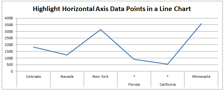
Horizontal Axis Label Highlight in an Excel Line Chart ...
How to add axis label to chart in Excel? - ExtendOffice Select the chart that you want to add axis label. 2. Navigate to Chart Tools Layout tab, and then click Axis Titles, see screenshot: 3.
Excel axis labels - supercategory — storytelling with data
Change axis labels in a chart in Office - support.microsoft.com In charts, axis labels are shown below the horizontal (also known as category) axis, next to the vertical (also known as value) axis, and, in a 3-D chart, next to the depth axis. The chart uses text from your source data for axis labels. To change the label, you can change the text in the source data.
How to customize chart axis
Excel 2019 will not use text column as X-axis labels Excel 2019 will not use text column as X-axis labels No matter what I do or which chart type I choose, when I try to plot numerical values (Y) against a column formatted as "text" (X), the program always converts the words in the text cells into ordinal integers as its x-axis labels. I have never had this problem with previous versions of Excel.
How to Change Axis Values in Excel | Excelchat
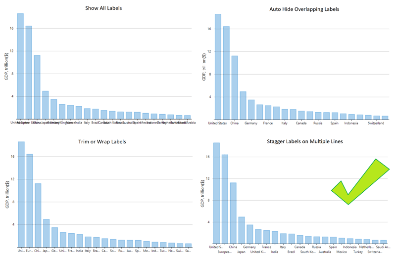
HOW TO STAGGER AXIS LABELS IN EXCEL - simplexCT HOW TO STAGGER AXIS LABELS IN EXCEL 21. In the chart, right click the Horizontal (Category) Axis and on the shortcut menu click Format Axis. 22. In the Format Axis pane, under Labels, set the Labels Position to None. 23. Click the Fill & Line icon and select Solid Line under Line and set the Color to Black and the Width to 1.5. 24.

Add or remove titles in a chart
Two-Level Axis Labels (Microsoft Excel) - tips Excel automatically recognizes that you have two rows being used for the X-axis labels, and formats the chart correctly. (See Figure 1.) Since the X-axis labels appear beneath the chart data, the order of the label rows is reversed—exactly as mentioned at the first of this tip. Figure 1. Two-level axis labels are created automatically by Excel.

Changing Axis Labels in Excel 2016 for Mac - Microsoft Community
Chart Axis - Use Text Instead of Numbers - Automate Excel Change Labels. While clicking the new series, select the + Sign in the top right of the graph. Select Data Labels. Click on Arrow and click Left. 4. Double click on each Y Axis line type = in the formula bar and select the cell to reference. 5. Click on the Series and Change the Fill and outline to No Fill. 6.
Add or remove a secondary axis in a chart in Excel
Excel Chart: Horizontal Axis Labels won't update I created the data set in Excel 2016, selected the data and inserted a line chart. I sent one line to the secondary axis. The X axis still shows the correct labels. I sent the other line to the secondary axis and brought the first line back to the primary axis. The X axis labels are still correct. In short, I cannot reproduce the problem.

Excel: How to create a dual axis chart with overlapping bars ...
Excel tutorial: How to create a multi level axis To straighten out the labels, I need to restructure the data. First, I'll sort by region and then by activity. Next, I'll remove the extra, unneeded entries from the region column. The goal is to create an outline that reflects what you want to see in the axis labels. Now you can see we have a multi level category axis.
Customize C# Chart Options - Axis, Labels, Grouping ...
Format Chart Axis in Excel - Axis Options Dec 14, 2021 · Thereafter, Axis options and Text options are the two sub panes of the format axis pane. Formatting Chart Axis in Excel – Axis Options : Sub Panes. There is some more sub-division of panes in the axis options named: Fill and Line, Effects, Size and properties, Axis Options. We have worked with the Fill and Line, Effects in our previous blog.

charts - Excel line diagram x-axis labels by week - Super User
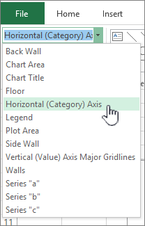
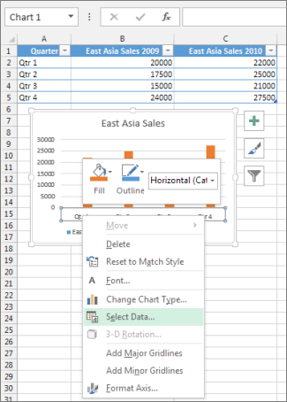
Change the display of chart axes - support.microsoft.com On the Format tab, in the Current Selection group, click the arrow in the Chart Elements box, and then click the horizontal (category) axis. On the Design tab, in the Data group, click Select Data. In the Select Data Source dialog box, under Horizontal (Categories) Axis Labels, click Edit.

Stagger long axis labels and make one label stand out in an ...
Broken Y Axis in an Excel Chart - Peltier Tech 18.11.2011 · This link shows a broken line graph but didn’t say anything about how to draw the broken line graph in excel. ... every Excel forum and blog he could find between 2003 and 2008 posting the link to his website on how to break the axis in an Excel graph. He’s basically been the equivalent of a little kid bragging about his new basketball and asking us to play a game for 5 …

How to Add Axis Labels in Excel Charts - Step-by-Step (2022)
Line Chart Examples | Top 7 Types of Line Charts in Excel with … Line charts can display lines horizontally that consist of the horizontal X-axis, which is an independent axis because the values in the X-axis do not depend on anything. Typically, it would be time on the X-axis as it continues to move forward irrespective of anything) and the vertical Y-axis, which is the dependent axis because the values in the Y-axis will depend on the X-axis. …
Label Specific Excel Chart Axis Dates • My Online Training Hub
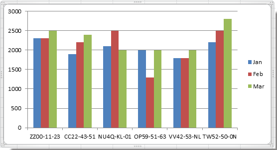
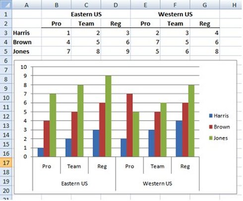
How to group (two-level) axis labels in a chart in Excel? - ExtendOffice (1) In Excel 2007 and 2010, clicking the PivotTable > PivotChart in the Tables group on the Insert Tab; (2) In Excel 2013, clicking the Pivot Chart > Pivot Chart in the Charts group on the Insert tab. 2. In the opening dialog box, check the Existing worksheet option, and then select a cell in current worksheet, and click the OK button. 3.
How to group (two-level) axis labels in a chart in Excel
How to Add Axis Labels in Excel Charts - Step-by-Step (2022) - Spreadsheeto How to add axis titles 1. Left-click the Excel chart. 2. Click the plus button in the upper right corner of the chart. 3. Click Axis Titles to put a checkmark in the axis title checkbox. This will display axis titles. 4. Click the added axis title text box to write your axis label.
Change axis labels in a chart
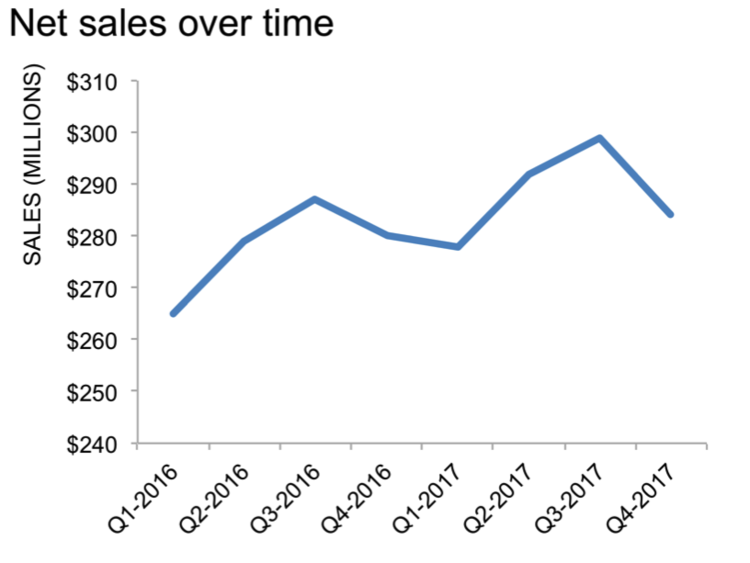
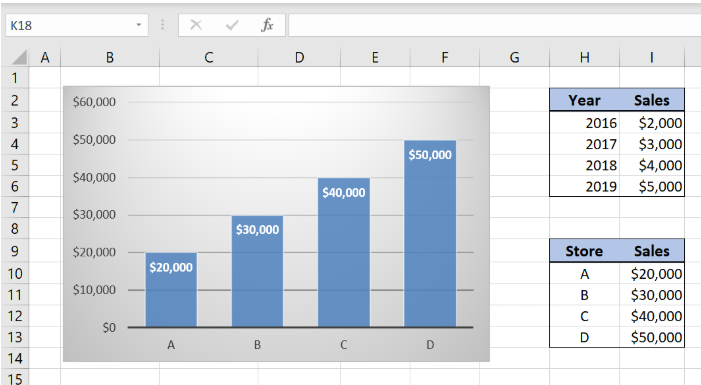
Change axis labels in a chart - support.microsoft.com Right-click the category labels you want to change, and click Select Data. In the Horizontal (Category) Axis Labels box, click Edit. In the Axis label range box, enter the labels you want to use, separated by commas. For example, type Quarter 1,Quarter 2,Quarter 3,Quarter 4. Change the format of text and numbers in labels

Change axis labels in a chart
3 Types of Line Graph/Chart: + [Examples & Excel Tutorial] - Formpl 20.04.2020 · Labels. Each axis on a line graph has a label that indicates what kind of data is represented in the graph. The X-axis describes the data points on the line and the y-axis shows the numeric value for each point on the line. We have 2 types of labels namely; the horizontal label and the vertical label. The horizontal label defines the data that is being described on the x …
How to rotate axis labels in chart in Excel?
Shorten Y Axis Labels On A Chart - How To Excel At Excel Right-click the Y axis (try right-clicking one of the labels) and choose Format Axis from the resulting context menu. Choose Number in the left pane. In Excel 2003, click the Number tab. Choose Custom from the Category list. Enter the custom format code £0,,\ m, as shown in Figure 2. In Excel 2007, click Add.
Change the display of chart axes
How to rotate axis labels in chart in Excel? - ExtendOffice If you are using Microsoft Excel 2013, you can rotate the axis labels with following steps: 1. Go to the chart and right click its axis labels you will rotate, and select the Format Axis from the context menu. 2.

How to wrap X axis labels in a chart in Excel?

How to Add Axis Labels in Excel Charts - Step-by-Step (2022)

Moving X-axis labels at the bottom of the chart below ...
How to Add Axis Titles in Excel
How To Add Axis Labels In Excel - BSUPERIOR
How to get rid of vertical lines in double labels on x-axis ...
Chart Elements

In an Excel chart, how do you craft X-axis labels with whole ...
How to customize axis labels
How to Add Axis Labels to a Chart in Excel | CustomGuide

Creating multiple y axis graph in excel 2007 – Yuval Ararat
X-Axis labels in excel graph are showing sequence of numbers ...
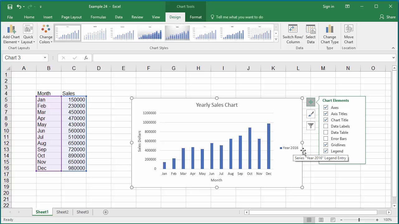
How to Change Elements of a Chart like Title, Axis Titles, Legend etc in Excel 2016

Individually Formatted Category Axis Labels - Peltier Tech
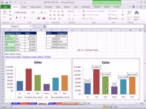
Excel Magic Trick 804: Chart Double Horizontal Axis Labels & VLOOKUP to Assign Sales Category

Two-Level Axis Labels (Microsoft Excel)
Post a Comment for "38 excel line graph axis labels"